Examples#
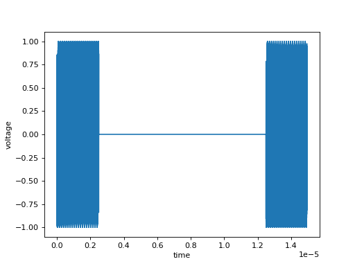
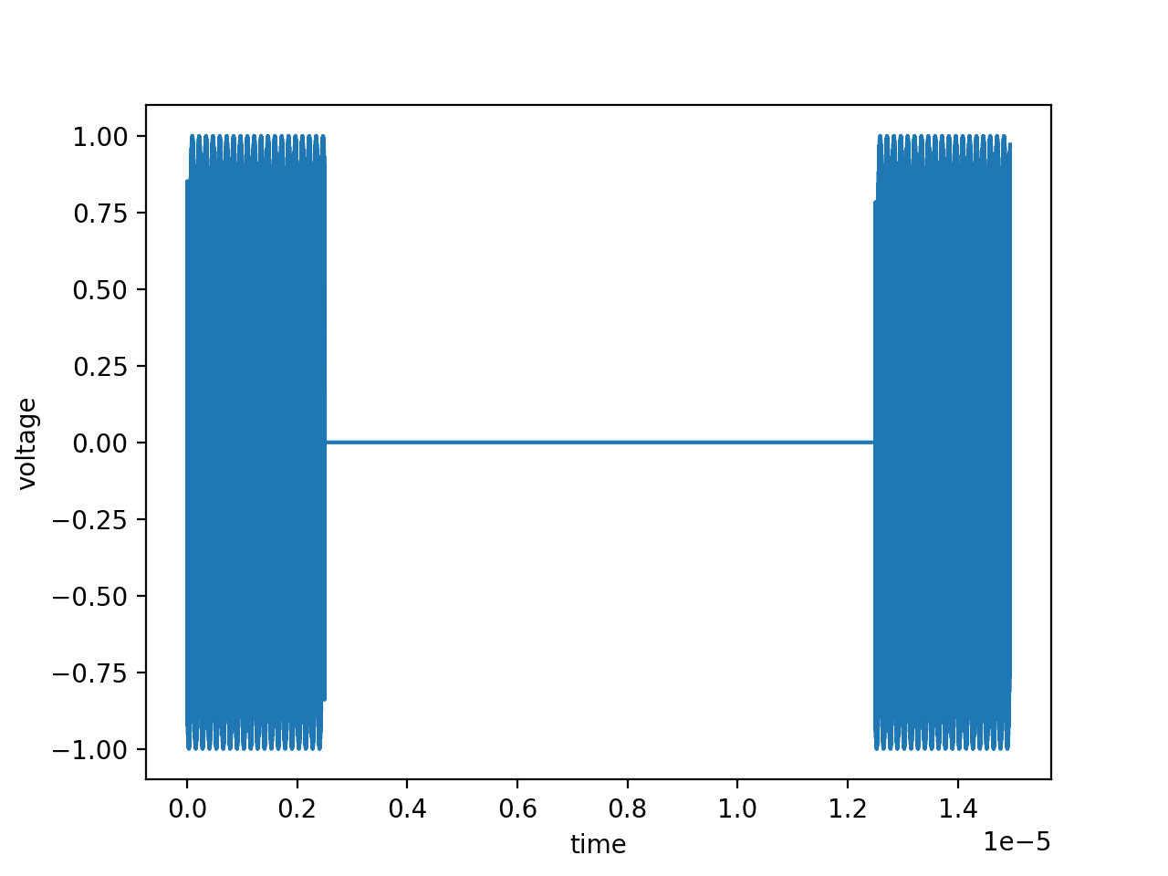
Ramsey Spectroscopy#
import WaveformConstructor
from scipy.constants import *
import matplotlib.pyplot as plt

# Define the parameters of the waveform
half_pi_time = 2.5 * micro # half pi time of the flopping.
amplitude = 1.0
frequency = WaveformConstructor.DefaultValues.carrier_freq + 1 * kilo # frequency of
phase = 0
ramsey_duration = 1 * 10 * micro # wait time of the Ramsey spectroscopy

# Create a waveform series. The waveform series consists of three waveforms:
# 1. A pi/2 pulse
# 2. A wait time
# 3. A pi/2 pulse
# The total time of the waveform series is the sum of the time of the three
# waveforms.
waveform_series = WaveformConstructor.WaveformSeries(
    [half_pi_time, ramsey_duration, half_pi_time],
    [
        WaveformConstructor.X(amplitude, frequency),
        WaveformConstructor.Zero(),
        WaveformConstructor.X(amplitude, frequency)
    ]
)

print("total time of the waveform:", waveform_series.total_time)

# Evaluate the waveform
t, v = waveform_series.waveform(sampling_rate=int(625 * mega))


# Visualize the waveform
plt.plot(t, v)
plt.xlabel("time")
plt.ylabel("voltage")
plt.show()
(Source code, png, hires.png, pdf)

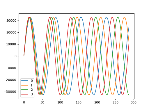
Scan Frequency#
import WaveformConstructor
from scipy.constants import *
import matplotlib.pyplot as plt
import numpy as np

# Define the parameters of the waveform
span = 2 * mega
freq = 10 * mega
num_point = 4
duration = 500 * nano

# Create a collection of waveforms
collection = []

# Create waveform series for each frequency
for freq in np.linspace(
    freq - span / 2,
    freq + span / 2,
    num_point
):
    waveform_series = WaveformConstructor.WaveformSeries(
        [duration],
        [
            WaveformConstructor.X(1, freq),
        ]
    )
    collection.append(waveform_series)

# Create a waveform factory with the collection of waveforms
factory = WaveformConstructor.WaveformFactory(collection,
        sampling_rate=WaveformConstructor.DefaultValues.sampling_rate)

# Sample the waveforms and plot them
for index, waveform_array in factory.pipeline():
    plt.plot(waveform_array, label=f"{index}")

plt.legend()
plt.show()
(Source code, png, hires.png, pdf)

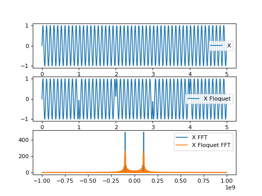
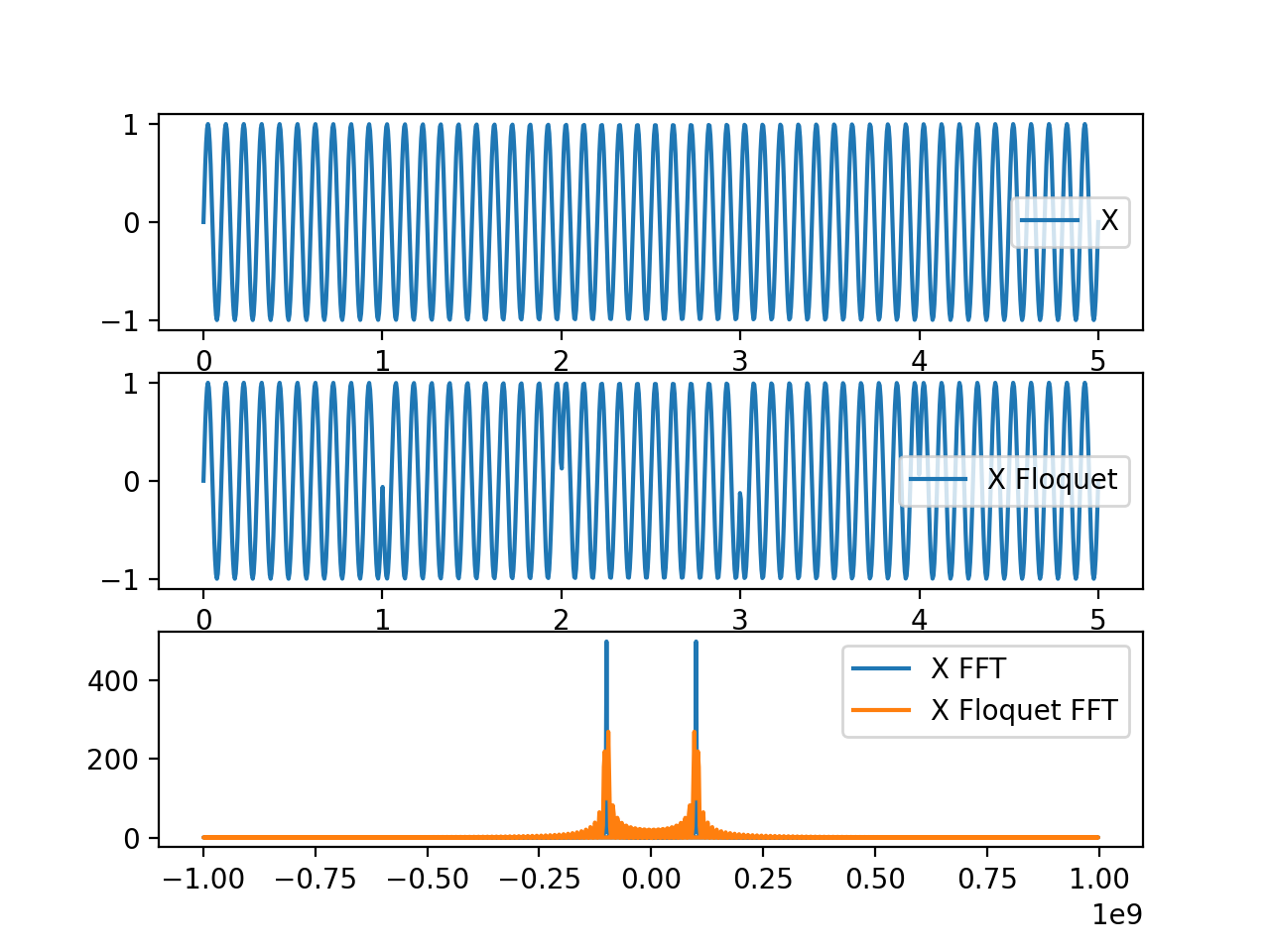
Floquet#
import WaveformConstructor
from scipy.constants import *
import matplotlib.pyplot as plt
import numpy as np

# Define the parameters of the waveform
span = 2 * mega
freq = 100 * mega
num_point = 4
duration = 500 * nano

t = np.linspace(0, duration, 1000)


x = WaveformConstructor.X(1, freq)(t)
x_floquet = WaveformConstructor.XFloquet(1, freq / 10, freq)(t)

# Visualize the waveform
plt.subplot(3, 1, 1)
plt.plot(t, x, label="X")
plt.legend()
plt.subplot(3, 1, 2)
plt.plot(t, x_floquet, label="X Floquet")
plt.legend()
plt.subplot(3, 1, 3)
f = np.fft.fftfreq(len(t), t[1] - t[0])
plt.plot(f, np.abs(np.fft.fft(x)), label="X FFT")
plt.plot(f, np.abs(np.fft.fft(x_floquet)), label="X Floquet FFT")

plt.legend()
plt.show()
(Source code, png, hires.png, pdf)

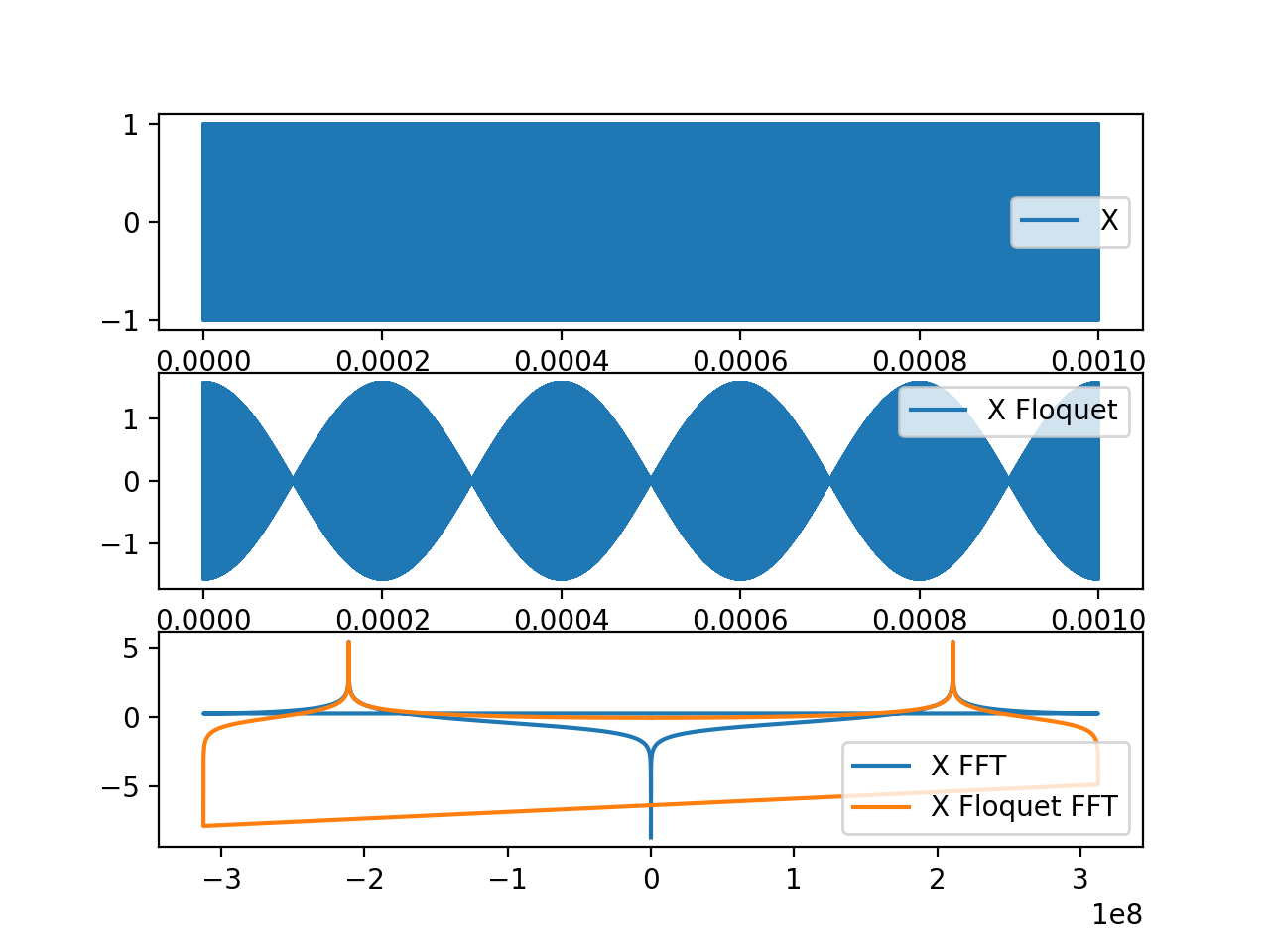
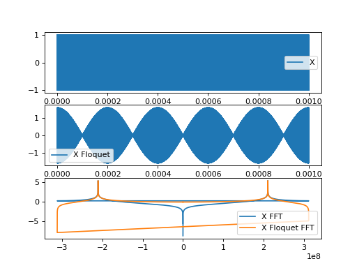
Floquet with Cosine Drive#
import WaveformConstructor
from scipy.constants import *
import matplotlib.pyplot as plt
import numpy as np

# Define the parameters of the waveform
span = 2 * mega
freq = 211 * mega
num_point = 4
duration = 1*milli

t = np.linspace(0, duration, int(duration*625*mega))


x = WaveformConstructor.X(1, freq)(t)
x_floquet = WaveformConstructor.XFloquetCosDrive(1, 5*kilo, freq)(t)

# Visualize the waveform
plt.subplot(3, 1, 1)
plt.plot(t, x, label="X")
plt.legend()
plt.subplot(3, 1, 2)
plt.plot(t, x_floquet, label="X Floquet")
plt.legend()
plt.subplot(3, 1, 3)
f = np.fft.fftfreq(len(t), t[1] - t[0])
plt.plot(f, np.log10(np.abs(np.fft.fft(x))), label="X FFT")
plt.plot(f, np.log10(np.abs(np.fft.fft(x_floquet))), label="X Floquet FFT")

plt.legend()
plt.show()
(Source code, png, hires.png, pdf)
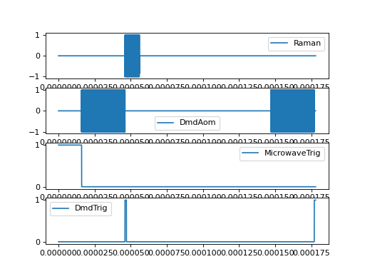
Zeeman Shelving#
import WaveformConstructor as wc
from scipy.constants import *
import matplotlib.pyplot as plt
import numpy as np
from enum import IntEnum

class Channel(IntEnum):
    Raman = 0
    DmdAom = 1
    MicrowaveTrig = 2
    DmdTrig = 3

mcc = wc.MultiChannelComposer(4, digital=[Channel.MicrowaveTrig, Channel.DmdTrig])

shelving_time = 16 * micro
dmd_pump_time = 30 * micro
raman_time = 10 * micro

trigger_on_time = 1 * micro
minimum_dmd_wait_time = 100 * micro # wait time before it is ready for the next frame


exp_waveform = wc.WaveformSeries(
    [raman_time],
    [wc.X(1)]
)

mcc.append_waveform(Channel.MicrowaveTrig, wc.On(), shelving_time)
mcc.sync()
mcc.append_waveform(Channel.DmdAom, wc.SineWave(1, 200 * mega, 0), dmd_pump_time)
mcc.sync()
mcc.append_series(Channel.Raman, exp_waveform)
# while doing the experiment, switch the dmd pattern in parallel
mcc.append_waveform(Channel.DmdTrig, wc.On(), trigger_on_time)
mcc.append_waveform(Channel.DmdTrig, wc.Off(), minimum_dmd_wait_time)
mcc.sync()
mcc.append_waveform(Channel.DmdAom, wc.SineWave(1, 200 * mega, 0), dmd_pump_time)
mcc.sync()
mcc.append_waveform(Channel.DmdTrig, wc.On(), trigger_on_time)
mcc.sync()


plt.figure()
plt.subplot(4, 1, 1)
plt.plot(*mcc.channel[Channel.Raman].waveform(), label="Raman")
plt.legend()
plt.subplot(4, 1, 2)
plt.plot(*mcc.channel[Channel.DmdAom].waveform(), label="DmdAom")
plt.legend()
plt.subplot(4, 1, 3)
plt.plot(*mcc.channel[Channel.MicrowaveTrig].waveform(), label="MicrowaveTrig")
plt.legend()
plt.subplot(4, 1, 4)
plt.plot(*mcc.channel[Channel.DmdTrig].waveform(), label="DmdTrig")
plt.legend()
plt.show()
(Source code, png, hires.png, pdf)
